%%%%%%%%%%%%%%%%%
% Problem Setup %
%%%%%%%%%%%%%%%%%

clear all
close all

% Physical constants
eps0 = 8.8541878e-12;
mu0  = 4e-7 * pi;
c0 = 299792458;

% Cell size
h = 0.0025;

% Waveguide dimensions
Lx = 0.040;
Ly = 0.0225;
Lz = 0.160;


% Number of cells in each direction
Nx = round(Lx / h);
Ny = round(Ly / h);
Nz = round(Lz / h);

% Length of time steps
Dt = h / (c0 * sqrt(3)); % Courant condition?

% Insignal data
t_max = 16e-9;
Nt    = ceil(t_max / Dt);
t     = (1:Nt)' * Dt;

f_min = 4e9;
f_max = 7e9;
f_mid = (f_max + f_min) / 2;
BWr   = (f_max - f_mid) / f_mid;
f     = ((0:Nt-1)'-floor(Nt/2)) / Nt / Dt;
s     = gauspuls(t-0.2e-8, f_mid, BWr, -12);

% Allocate field matrices
Ex = zeros(Nx,     Ny + 1, Nz + 1);
Ey = zeros(Nx + 1, Ny,     Nz + 1);
Ez = zeros(Nx + 1, Ny + 1, Nz    );

Hx = zeros(Nx + 1, Ny,     Nz    );
Hy = zeros(Nx    , Ny + 1, Nz    );
Hz = zeros(Nx    , Ny,     Nz + 1);

%%%%%%%%%%%%%%%%%%%%%%%%%%%%%%%%%%%%%
% Initiation of boundary conditions %
%%%%%%%%%%%%%%%%%%%%%%%%%%%%%%%%%%%%%
disp(sprintf('Initiate boundary conditions...'))
NumModesTE = 7; % 01 10 11 20 21 30 31
NumModesTM = 3; % 11 21 31
NumModes   = NumModesTE + NumModesTM;

disp(sprintf('  Compute TE modes'))
[ExTE, EyTE, K2TE] = ComputeTEModes(NumModesTE, Nx, Ny, h, h);
disp(sprintf('  Compute TM modes'))
[ExTM, EyTM, K2TM] = ComputeTMModes(NumModesTM, Nx, Ny, h, h);

ModalEx = [ExTE ExTM];
ModalEy = [EyTE EyTM];
ModalK2 = [K2TE K2TM];
ModalNm = sum(ModalEx.^2) + sum(ModalEy.^2); % Normalizing constants

clear ExTE EyTE ExTM EyTM

% Compute Impulse response for the propagating mode
IR   = zeros(Nt, NumModes);  % Impulse response
s1R  = zeros(Nt, NumModes);  % Reflected signal at z = Dz
s1   = zeros(Nt, NumModes);  % Total signal at z = 0
s2T  = zeros(Nt, NumModes);  % Transmitted signal at z = Lz - Dz
s2   = zeros(Nt, NumModes);  % Total signal at z = Lz

for k = 1:NumModes
  disp(sprintf('  Computing Impulse response for Mode %d', k))
  IR(:,k) = ComputeIR(Dt, h, Nt, ModalK2(k));
end

%%%%%%%%%%%%%%
% Main Loop. %
%%%%%%%%%%%%%%
disp(sprintf('Start time stepping...'))
% Set initial source boundary conditions
sEy = Ey(2:Nx, :, 2);
sEx = Ex(:, 2:Ny, 2);
sEy(:) = s(1) * ModalEy(:,1);
sEx(:) = s(1) * ModalEx(:,1);
Ey(2:Nx, :, 1) = sEy;
Ex(:, 2:Ny, 1) = sEx;
s1(1,1) = s(1);

CH = Dt / (h * mu0);
CE = Dt / (h * eps0);

ks = 400;
for k = 2:Nt

  % if k > 250 & k < 600
  %   figure(99)
  %   mesh(0:Nz, 0:Nx, squeeze(0.5*Ey(:,6,:))), axis equal, axis([0 Nz 0 Nx -6 6])
  %   caxis([-6 6]), view(145,30)
  %   title(num2str(k))
  %   drawnow
  % end



  %===================%
  % FDTD update loops %
  %===================%

  % -------------------------------------------------------------
  % | ADD FDTD UPDATE LOOPS                                     |
  % ----------------------------------------------------------  |
  %                                                          |  |
  %                                                         \    /
  %                                                          \  /
  %                                                           \/

    % Hx = zeros(Nx + 1, Ny,     Nz    );
    % Hy = zeros(Nx    , Ny + 1, Nz    );
    % Hz = zeros(Nx    , Ny,     Nz + 1);
    %
    % Ex = zeros(Nx,     Ny + 1, Nz + 1);
    % Ey = zeros(Nx + 1, Ny,     Nz + 1);
    % Ez = zeros(Nx + 1, Ny + 1, Nz    );

    % diff(A, n, dim) differentiates matrix A by order n over dimension dim. Eg. dHz/dy = diff(Hz(:,:,2:Nz), 1, 2). Obs! Hz(:,:,2:Nz) because boundaries are constant 0 in this problem.

  Hx = Hx + CH * (diff(Ey,1,3) - diff(Ez,1,2));
  Hy = Hy + CH * (diff(Ez,1,1) - diff(Ex,1,3));
  Hz = Hz + CH * (diff(Ex,1,2) - diff(Ey,1,1));

  Ex(: ,2:Ny, 2:Nz) = Ex(: ,2:Ny, 2:Nz) + CE * (diff(Hz(:,:,2:Nz),1,2) - diff(Hy(:,2:Ny,:),1,3));
  Ey(2:Nx ,: ,2:Nz) = Ey(2:Nx ,: ,2:Nz) + CE * (diff(Hx(2:Nx,:,:),1,3) - diff(Hz(:,:,2:Nz),1,1));
  Ez(2:Nx, 2:Ny, :) = Ez(2:Nx, 2:Ny, :) + CE * (diff(Hy(:,2:Ny,:),1,1) - diff(Hx(2:Nx,:,:),1,2));


  %                                                           /\
  %                                                          /  \
  %                                                         /    \
  %                                                          |  |
  % ----------------------------------------------------------  |
  % |                                                           |
  % -------------------------------------------------------------



  %==========================%
  % Metal Boudary Conditions %
  %==========================%

  % -------------------------------------------------------------
  % | ADD METAL OBJECTS FOR FILTERING                           |
  % ----------------------------------------------------------  |
  %                                                          |  |
  %                                                         \    /
  %                                                          \  /
  %                                                           \/

   % Set E-components to zero at new walls in narrow section.
   % b = 6cm , a = w = 4cm, d = 3cm

    a = 4e-2; b = 6e-2; d = 3e-2; w = a;


    x_grid = linspace(0, Lx, Nx+1);
    y_grid = linspace(0, Ly, Ny+1);
    z_grid = linspace(0, Lz, Nz+1);
    % Indices that correspond to PEC boundary, including boundary wall
    x_narrow = [find(x_grid <= (Lx-d)/2), find(x_grid >= w-(Lx-d)/2)];
    z_narrow = find(z_grid >= b & z_grid <= a+b);

    % Apply metal boundary conditions by setting E-components to zero

    % Surfaces inwards towards middle
    for x = [find(x_grid == 5e-3), find(x_grid == 35e-3) ]
        Ez(x, :, z_narrow) = 0;
        Ey(x, :, z_narrow) = 0;
    end

    % Surfaces outwards towards each port
    for z = [find(z_grid == b), find(z_grid == b+a)]
        Ex([1,2,end-1,end], :, z) = 0;
        Ey([1,2,end-1,end], :, z) = 0;
    end

    %
    % plot3([find(z_grid == b),find(z_grid == b)], [0, Nx], [0,0], "k")

  %                                                           /\
  %                                                          /  \
  %                                                         /    \
  %                                                          |  |
  % ----------------------------------------------------------  |
  % |                                                           |
  % -------------------------------------------------------------



  %==============================%
  % Boundary Conditions at Z = 0 %
  %==============================%

  % Extract transverse fields at z = dz %
  sEy = Ey(2:Nx, :, 2);
  sEx = Ex(:, 2:Ny, 2);

  % Compute modal voltages %
  s1R(k,:) = (sEy(:)' * ModalEy + sEx(:)' * ModalEx) ./ ModalNm;

  % The reflected modal amplitude at z = Dz is the difference between the
  % total modal amplitude and that of the incoming wave. The amplitude of
  % the incoming wave at z = Dz is a convolution of the insignal at z = 0
  % and the impulse response of the wave guide.
  s1R(k,1) = s1R(k,1) - s(1:k-1)' * IR(k-1:-1:1,1);

  % Port Amplitude: sum of insignal and convolution of the reflected
  % signal at z = Dz with the impulse response
  for l = 1:NumModes
    s1(k,l) = s1R(1:k-1, l)' * IR(k-1:-1:1, l);
  end
  s1(k,1) = s1(k,1) + s(k);

  % Set port 1  boundary conditions %
  sEy(:) = ModalEy * s1(k,:)';
  sEx(:) = ModalEx * s1(k,:)';
  Ey(2:Nx,:,1) = sEy;
  Ex(:,2:Ny,1) = sEx;

  %===============================%
  % Boundary Conditions at Z = Lz %
  %===============================%

  % Extract transverse fields at z = Lz - Dz %
  sEy = Ey(2:Nx, :, Nz);
  sEx = Ex(:, 2:Ny, Nz);

  % Compute modal voltage at z = Dz
  s2T(k,:) = (sEy(:)' * ModalEy + sEx(:)' * ModalEx) ./ ModalNm;

  % Port Amplitude
  for l = 1:NumModes
    s2(k,l) = s2T(1:k-1, l)' * IR(k-1:-1:1, l);
  end

  % Set port 2  boundary conditions %
  sEy(:) = ModalEy * s2(k,:)';
  sEx(:) = ModalEx * s2(k,:)';
  Ey(2:Nx,:,Nz+1) = sEy;
  Ex(:,2:Ny,Nz+1) = sEx;

  if(mod(k,100) == 0)
    disp(sprintf('  step %5d of %5d', k, Nt))
  end

end;

% remove the incoming sigland from the total signal at port 1.
s1(:,1) = s1(:,1) - s;



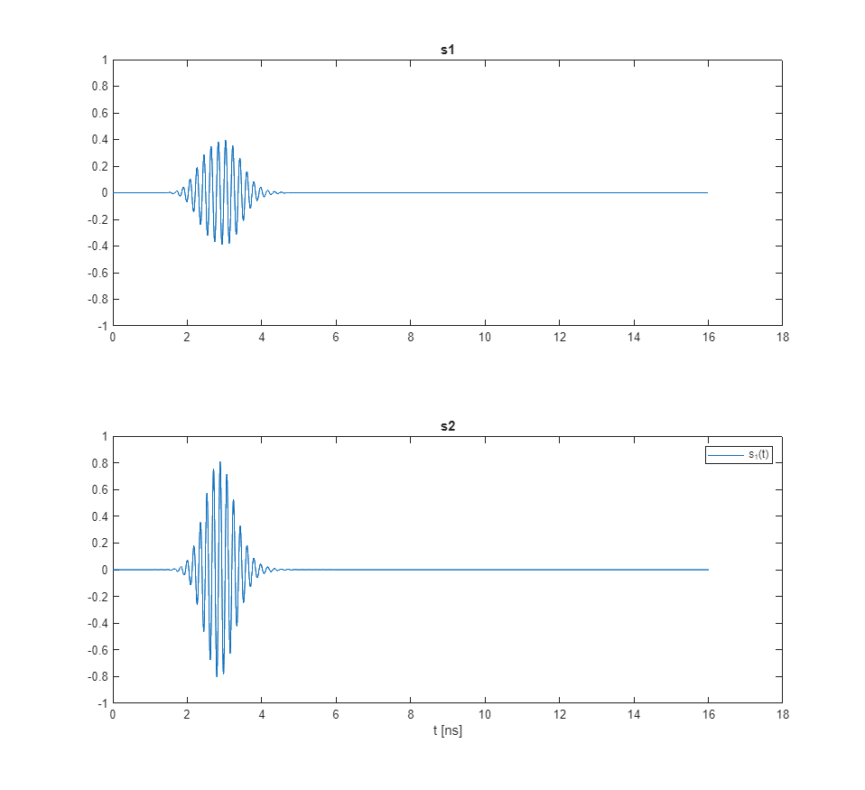
figure(1)
tiledlayout(2,1)
nexttile
T = t*1e9;
plot(T,s1(:,1))
title("s1")
ylim([-1, 1])
nexttile
plot(T,s2(:,1))
legend('s_1(t)','s_2(t)')
xlabel('t [ns]');
ylim([-1, 1])
title("s2")





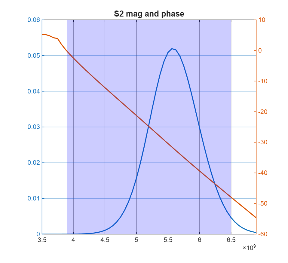
figure
[f, S2, S2_phase] = (myfft(Dt, s2(:,1), 1:Nt));
yyaxis left;
plot(f, S2, "DisplayName","S2")
yyaxis right;
plot(f, unwrap(S2_phase(1:length(S2_phase)/2+1)))
title("S2 mag and phase")
xlim([3.5e9, 6.9e9])
prettify_axes(gca, 3.9e9, 6.5e9)

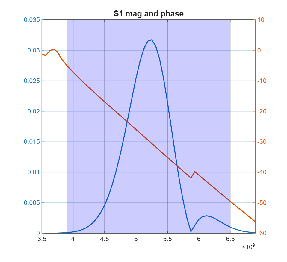
figure
[f, S1, S1_phase] = (myfft(Dt, s1(:,1), 1:Nt));
yyaxis left;
plot(f, S1, "DisplayName","S1")
yyaxis right;
plot(f, unwrap(S1_phase(1:length(S1_phase)/2+1)))
title("S1 mag and phase")
xlim([3.5e9, 6.9e9])
prettify_axes(gca, 3.9e9, 6.5e9)

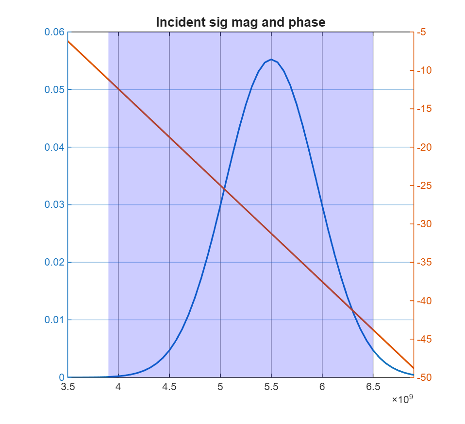
figure
[f, S, S_phase] = myfft(Dt, s, 1:Nt); % gaussian pulse input
yyaxis left;
plot(f, S, "DisplayName","S")
yyaxis right;
plot(f, unwrap(S_phase(1:length(S_phase)/2+1)))
title("Incident sig mag and phase")
xlim([3.5e9, 6.9e9])
prettify_axes(gca, 3.9e9, 6.5e9)



% -------------------------------------------------------------
% | ADD SCATTERING PARAMETERS AS FUNCTION OF FREQUENCY        |
% ----------------------------------------------------------  |
%                                                          |  |
%                                                         \    /
%                                                          \  /
%
%

f_of_interest = find(f>3e9 & f<7e9);

S11 = (S1./S);
S21 = (S2./S);
S21_phase = (S2_phase - S_phase);
S11_phase = S1_phase - S_phase;




%                                                           /\
%                                                          /  \
%                                                         /    \
%                                                          |  |
% ----------------------------------------------------------  |
% |                                                           |
% -------------------------------------------------------------


% timevec = 1:Nt
function [f, mag, phase] =  myfft(Dt, signal, timevec)
    Fs = 1/Dt;
    L = length(signal); % same as for s2
    ts = timevec; % time vector
    Y = fft(signal);
    P2 = abs(Y/L);
    P1 = P2(1:L/2+1);
    P1(2:end-1) = 2*P1(2:end-1);
    f = Fs/L*(0:L/2);


    mag = P1;
    phase = angle(Y);

end

Initiate boundary conditions...
  Compute TE modes
  Compute TM modes
  Computing Impulse response for Mode 1
  Computing Impulse response for Mode 2
  Computing Impulse response for Mode 3
  Computing Impulse response for Mode 4
  Computing Impulse response for Mode 5
  Computing Impulse response for Mode 6
  Computing Impulse response for Mode 7
  Computing Impulse response for Mode 8
  Computing Impulse response for Mode 9
  Computing Impulse response for Mode 10
Start time stepping...
  step   100 of  3324
  step   200 of  3324
  step   300 of  3324
  step   400 of  3324
  step   500 of  3324
  step   600 of  3324
  step   700 of  3324
  step   800 of  3324
  step   900 of  3324
  step  1000 of  3324
  step  1100 of  3324
  step  1200 of  3324
  step  1300 of  3324
  step  1400 of  3324
  step  1500 of  3324
  step  1600 of  3324
  step  1700 of  3324
  step  1800 of  3324
  step  1900 of  3324
  step  2000 of  3324
  step  2100 of  3324
  step  2200 of  3324
  step  2300 of  3324
  step  2400 of  3324
  step  2500 of  3324
  step  2600 of  3324
  step  2700 of  3324
  step  2800 of  3324
  step  2900 of  3324
  step  3000 of  3324
  step  3100 of  3324
  step  3200 of  3324
  step  3300 of  3324
Warning: Ignoring extra legend entries. 

Published with MATLAB® R2025b